Microsoft Excel 2013 Keyboard Shortcut keys

Microsoft Excel 2013 Keyboard Shortcut keys from custom guide online training.

How to add excel online to your google chrome app store ??

how to insert formula in blank rows/column in excel 2007,2010

Hi Friends, after a little break of heavy work i come back to update my blog again. today will check how to insert formula's in blank rows & columns in between of large data.

This will help to complete your task quickly with single minute. lets go inside the How to's.

These are the simple steps to insert formulas in blank columns/rows. you can check the image for
explained view.

EXCEL SHORTCUT KEYS FOR NAVIGATION

Make easy and quick  navigation by using this keys in your excel

Previous sheet
CTRL + Page Up
Next sheet
CTRL + Page Down
Launch GO TO Dialog (from here you can select special or jump to a cell or range)
F5
Go to top left (will go to top left of freezed pane if set)
CTRL + Home
Go to last non-blank cell
CTRL + end
Go to previous sheet
CTRL + PgUp
Go to next sheet
CTRL + PgDn
Print
CTRL + p
Toggle between workbooks in a given session of excel.
CTRL + TAB

Save the below image for your desktop use.

EXCEL SHORTCUT KEYS FOR SELECTION

Use this shortcut keys for Selection in your Excel.
 

Select the whole column

CTRL + SPACE

Select the whole row

SHIFT + SPACE

Select table

SHIFT + CTRL + SPACE bar

Save

CTRL + s

Select visible cells only

ALT + ;

Select entire region

CTRL + A

Select range from start cell to far left

SHIFT + Home

Select range from start cell to end in direction of arrow

SHIFT + End + arrow

Select a continuous range of data (e.g. pivot), no matter where your cursor is.

CTRL + *

Select blank cells

F5 + ALT + S + K + ENTER

Select all cells with comments

CTRL + SHIFT + O

Select all cells that are directly or indirectly referred to by formulas in the selection

CTRL + SHIFT + {

Select all cells with formulas that refer directly or indirectly to the active cell

CTRL + SHIFT + }

Selects all the way to a1 from cursor position

CTRL + SHIFT + HOME

Select cells in the direction of arrow

CTRL + SHIFT + Arrow

Save the below image for your desktop use.

How to copy and paste image's in excel using shortcutKeys

Here some useful tips to copy and paste images in your excel sheet.

1. Click on the image Right Click => copy => paste in next cell.

2. Use Keyboard shortcut keys Ctrl + C for (copy) Ctrl + V for (paste)

3. Click on the image hold Ctrl + Drag with mouse.

How to insert image/picture into comment box in excel

Learning excel is very interesting for me.everyday i must try to learn something new in excel.
Try this simple trick in your excel file to impress your boss.

Here learn how to insert image into comment box in your excel data sheet.i used for this trick chandoo's the  legend in Microsoft Excel's New podcast image to insert in comment box.you can try your image's or some screenshots as your wish.

All you have to do is,

1. Open your Spreadsheet and click the cell where you want to add comment.
2. Remove your system name in comment box.
3. Right click with your mouse,add comment Box.
4. Right click again show/hide comments.
5. Click right hover on the comment box,select Format comment.
6. Go to colours & lines,select Fill effects.
7. Go to picture,click on select picture.
8. Select your image and click ok.
9. Maximize your comment box by using your mouse.

Delete Blank Rows/columns in excel large list with in minutes / seconds(works in Excel 2003,2007,2010)

Quick Tip : Delete Blank Rows/columns in excel large list with in minutes / seconds
 
         Preparing long list data from raw report pulled from software,bit difficult to compiles fast.
There are such a way to this activity like :

• Select blank rows/columns one by one and delete it which take more time to finish.
• Using Filter menu and Sort blanks, where you need to work again to alphabet the list.

Forget about these time consuming & Double work activity,just follow the steps to finish your work
like a lighting fast....

These are the steps to follow and check below attached pictorial too.

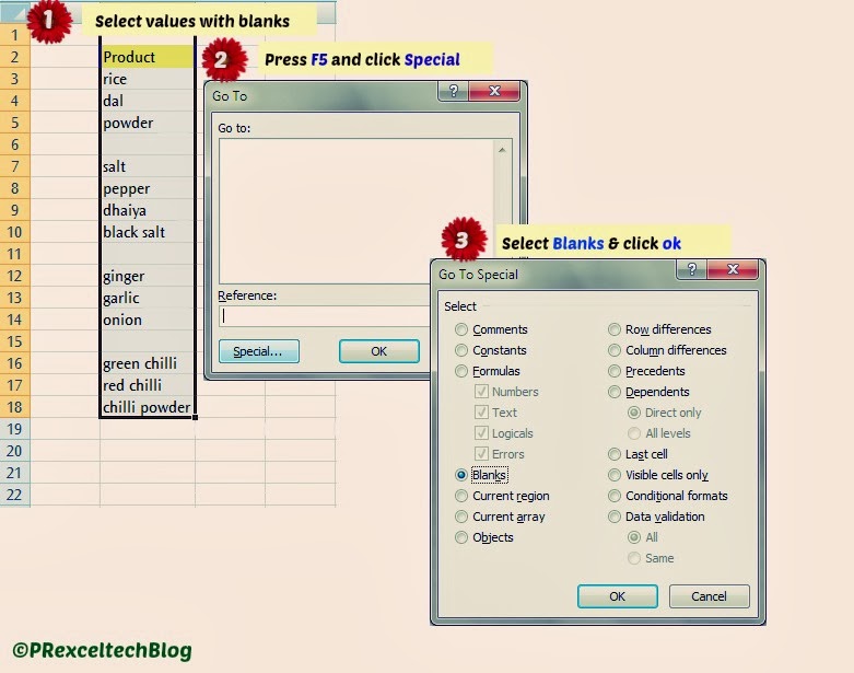
1. Select your Values with blanks.
2. Press F5(Go to Special)  and click special.
3. Select blanks and click OK.
4. now you can see all the empty cells are selected.
5. Delete blank cells by using Alt => h + d + r (or) Go to home => Delete cells=> Delete sheet rows.

 

 

  

How to insert division symbol in excel

Hello Friends, this month will be the end for closing year for accounting & finance. so we need to do types of reports to compare last year and this year flow.

Especially for Accounts & sales they need to do comparison,so lets give them a Quick tip to improve their reports.



Just hold your Alt key and type 0247 to get Division symbol.



  

Compare Two lists with easy and fun way by using Conditional Formatting

Hello Excel Geeks, Its a month end time for us, probably i think you guys started  to compare your  data sheets with previous month files. Learn this simple function and cut your work time in comparing two sheets (or) lists.

This Function Works only Excel 2007 or later versions only.Note : Most of us using Excel 2007+, only.

This is a beautiful and dead-simple way to compare lists in excel. try this and put me a comment below how it works.

A dead-simple and fun way to compare two lists in excel

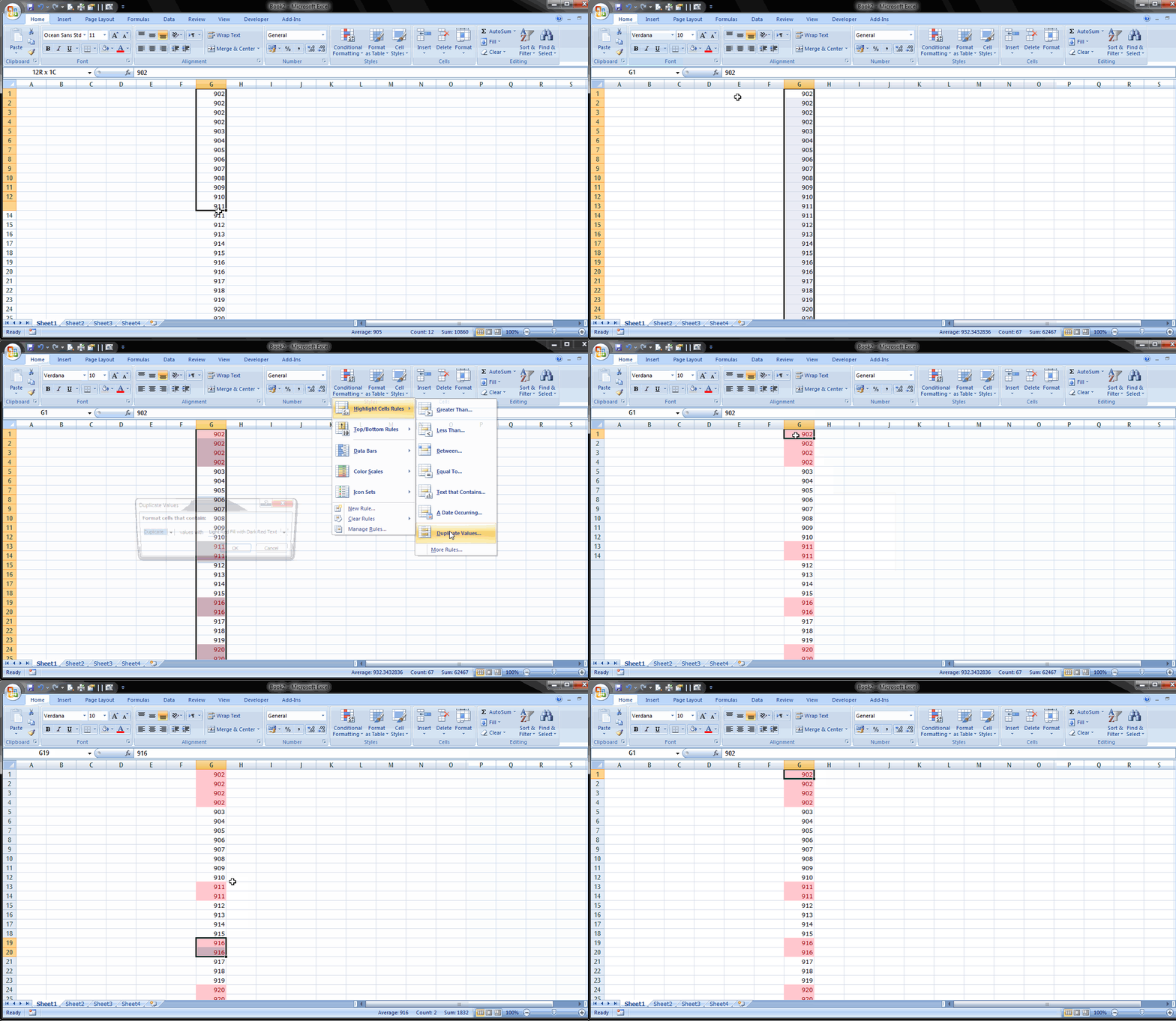
1. Select cells in the both lists (Select first list hold Ctrl key to select second list)
2. Go to Home tab click Conditional Formatting=> Highlight cells rules=>Duplicate values=>select unique (or) duplicate as you require.
3. Click OK.
4. Thats All.

How to change Rules colour in Duplicate values

1. Just follow the above steps same before click ok just change colour bye changing here =>Values with=> with default colours or if you need custom colour.

How to Remove Rules for selected lists

1. Here the steps to clear (remove) rules for selected lists
2. Select cells in the both lists (Select first list hold Ctrl key to select second list)
3. Go to Home tab click Conditional Formatting=> Clear Rules=>Clear Rules from selected cells.
4. Thats All.

How to Change your Excel spreadsheet background by using your own image /How to add a custom Background Image in Excel

Hello Everyone,Today i am going to explain how to change your spreadsheet background with your own image.follow the steps in picture below & mainly it is useful for professional guy who's submitting the spreadsheet to their boss.here i have just shown example with this month calender,you can follow the same steps for your excel sheet.

Now lets start the steps (Follow flower for step by step) :

Fix  your data to change background

Select your shape

Change shape colour with shape fill and right click select format shape.

Go to fill select file to insert picture.

Right click with your mouse again go to size and properties

Select the options given below (print object) is must

Again go to format shape => fill Change the transparency

Finally Check with print preview view

Hope you guys understood also check my video here

How to change Case-sensitive in Ms.Excel/how to change words into upper (or) lower case in excel

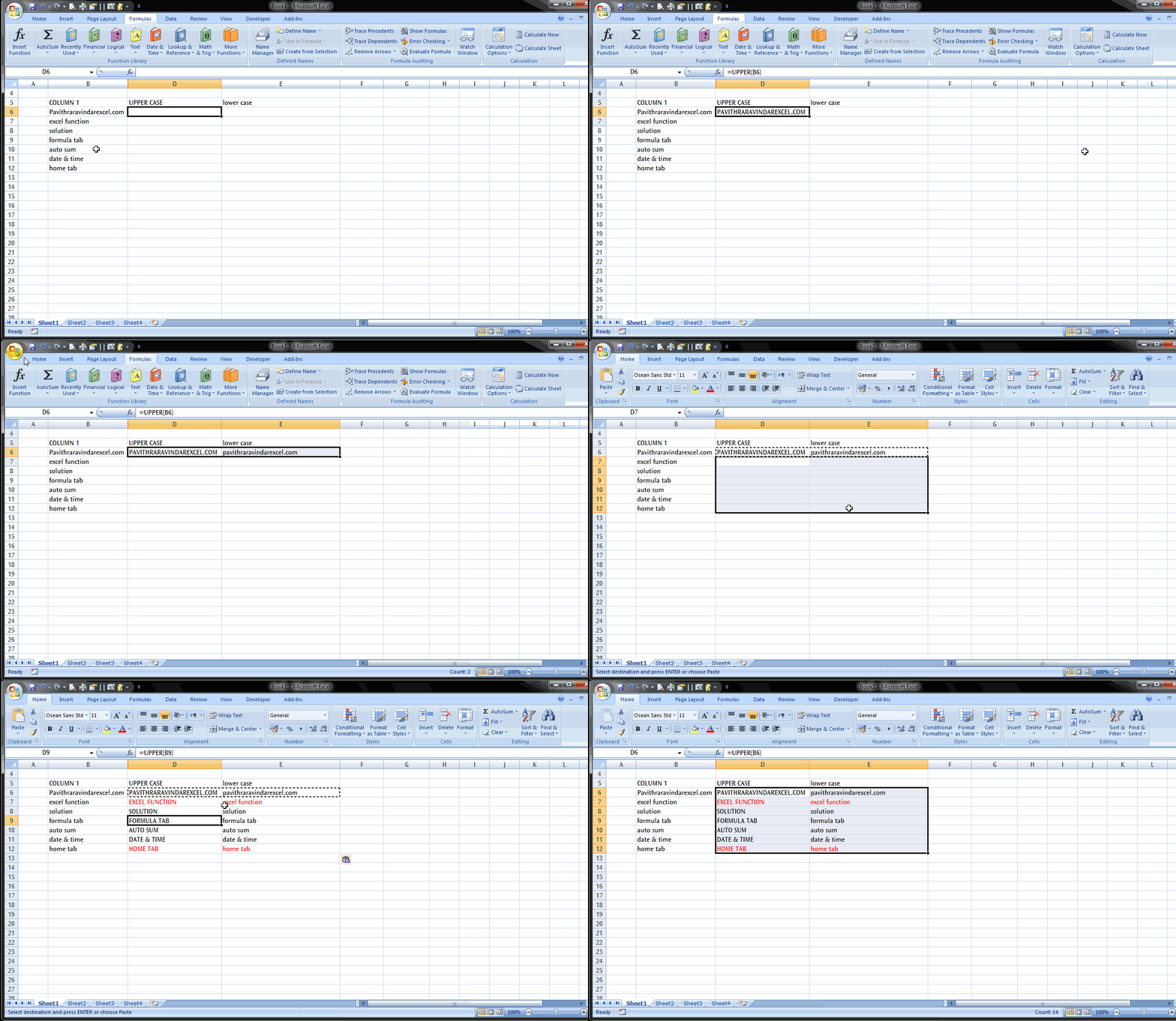
Hello Guys, Today i am going to explain about Case-Sensitive in Microsoft Excel.Before that i want say you  in Microsoft word there is an option to change the characters in to Uppercase (or) Lowercase. check the figure right now below.

But in excel we need to use formula to change Uppercase to Lowercase & the same for Lowercase to Uppercase.its a very simple formula to kept in memory.below  check the below animated image to learn how i use those formulas to change Case-Sensitive.

Hope you guys are understood sure.let me know about your thoughts.put a comment below.

How to research (or) key (or) word search in excel 2007?

Hi Guys,Want to research a word in microsoft excel ???. No need to go google & dictionary for search.just go to Review Tab & click research thats all.your excel will open a dictionary for you.

Click here for video
Open your excel Go To Review Tab & Proffing Group.

Just follow the  How To's (arrow marks) in the picture to know more :

Here check the below image to change the research settings. you can research about your text in Bing Right from from your Ms.Excel Workbook.

Change the Translation Options per your requirement.

Thanks for your time to spend on this post. I hope you guys understood.please put a comment below.

How to check duplicate values with conditional formatting in excel 2007

Check out the Gif image given below to learn (how to check duplicate values with conditional formatting
in excel 2007.

How to Find & Remove Duplicate Records in Excel 2007( How To's in youTube )

How to Find & Remove Duplicate Records in Excel 2007

When you love Excel, excel formulas will simply easy for you to access.As a inventory analyst i use to do this function to find duplicate entries in my inventory records.this function will helpful for people who are in the field accounting,inventory,etc .

This is a simple step to find & remove duplicate values or names in your data sheet,you can watch my video to learn this or just check follow the below steps.

Select your data 

Go to Data (Alt+ A) select Remove duplicates (M)

Select Continue with the current selection (Alt + C)

Select All (Alt + A)

Finally your data will look a like (here i have shown first & last name separately)

How to Split names & values by using the Convert Text to Columns wizard in excel 2007

What is Text to columns : 

Separate the contents of one excel cell into separate columns. For example,you can separate a column of full names into separate first & last name columns.

In word,use this feature to convert the selected text into a table,splitting the text into columns  at each comma,period,or other character you specify.

Simply watch this video in full screen mode you will get to know how to do this easily.

How to setup No of recent documents in excel 2007

Hello, let us look how to setup number of recent documents should show in your excel start menu.its just simple thing to do it, before that we need to know why we require this recent documents & what is the use of it.

once you open your workbook it will store in your recent documents until you delete your recent documents
history in your computer,it can be useful to you to open in one click, just you need to go start menu in your excel you can see the recent documents list, there you can pick up the excel file which you opened in previously. no need to go & search the folder where you stored the files. hope you understood.

lets start to know how to set recent documents history.

1. Go to your excel workbook. 
2. Click Start Menu = excel options = advanced = display = 
3. show this number of recent documents (10 )
4. save it.

Learn how to use clipboard group in excel 2007 Home Tab ???

Figure.1

Learn how to use clipboard group in excel 2007 :

Figure 2 

Shortcut Keys for Clipboard : ( To go Home Tab Open excel Alt + H )

• Cut - Ctrl + X
• Copy - Ctrl + C
• Paste - Ctrl + V
• For Paste Shortcut see figure 2